前言:
以斯坦福cs231n課程的python編程任務(wù)為主線,展開對該課程主要內(nèi)容的理解和部分?jǐn)?shù)學(xué)推導(dǎo)。該課程相關(guān)筆記參考自知乎-CS231n官方筆記授權(quán)翻譯總集篇發(fā)布課程材料和事例參考自-cs231n
本章為線性分類器的softmax講解,緊接上章的SVM,其中涉及到的一些線性分類器的知識已經(jīng)在上章說明,本次便不再贅述。cs231n課程作業(yè)assignment1(SVM)
SoftMax分類器簡介:
Softmax和SVM同屬于線性分類器,主要的區(qū)別在于Softmax的損失函數(shù)與SVM的損失函數(shù)的不同。Softmax分類器就可以理解為邏輯回歸分類器面對多個分類的一般化歸納。SVM將輸出f(x_i,W)作為每個分類的評分,而Softmax的輸出的是評分所占的比重,這樣顯得更加直觀。
在Softmax分類器中,函數(shù)映射f(x_i;W)=Wx_i保持不變,但將這些評分值視為每個分類的未歸一化的對數(shù)概率,并且將折葉損失(hinge loss)替換為交叉熵?fù)p失(cross-entropy loss)。公式如下:
)
或
在上式中,使用f_j來表示分類評分向量中f的第j個元素個,數(shù)據(jù)集的損失值是數(shù)據(jù)集中所有樣本數(shù)據(jù)的損失值的均值與正則化損失R(W)之和。其中Softmax函數(shù)為:
 = \frac{e{z_j}}{\sum_ke{f_j}})
其輸入值是一個向量,向量中元素為任意實數(shù)的評分值(z中的),函數(shù)對其進行壓縮,輸出一個向量,其中每個元素值在0到1之間,且所有元素之和為1。
除了損失函數(shù)不同,其他的操作與SVM基本相同,進一步的講,SVM分類器使用的是折葉損失(hinge loss),而Softmax使用的是交叉熵?fù)p失(corss-entropy loss),本質(zhì)上都屬于線性分類器的一種。
Softmax與SVM比較:
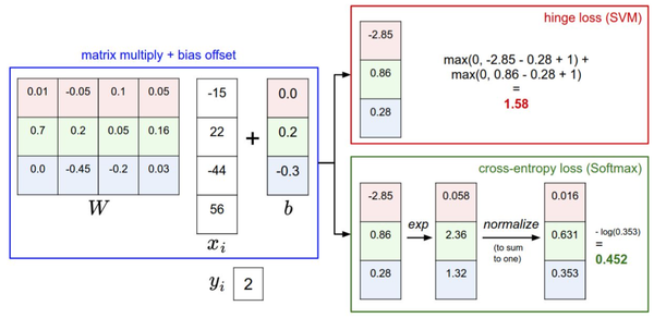
針對一個數(shù)據(jù)點,SVM和Softmax分類器的不同處理方式的例子。兩個分類器都計算了同樣的分值。不同之處在于對$f$分值的解釋:SVM分類器將它們看做是分類評分,它的損失函數(shù)鼓勵正確的分類(本例中是藍色的類別2)的分值比其他分類的分值高出至少一個邊界值。Softmax分類器將這些數(shù)值看做是每個分類沒有歸一化的對數(shù)概率,鼓勵正確分類的歸一化的對數(shù)概率變高,其余的變低。SVM的最終的損失值是1.58,Softmax的最終的損失值是0.452,但要注意這兩個數(shù)值沒有可比性。只在給定同樣數(shù)據(jù),在同樣的分類器的損失值計算中,它們才有意義。
在實際使用中,SVM和Softmax經(jīng)常是相似的:通常說來,兩種分類器的表現(xiàn)差別很小,不同的人對于哪個分類器更好有不同的看法。相對于Softmax分類器,SVM更加“局部目標(biāo)化(local objective)”,這既可以看做是一個特性,也可以看做是一個劣勢。考慮一個評分是[10, -2, 3]的數(shù)據(jù),其中第一個分類是正確的。那么一個SVM(&$Delta =1$)會看到正確分類相較于不正確分類,已經(jīng)得到了比邊界值還要高的分?jǐn)?shù),它就會認(rèn)為損失值是0。SVM對于數(shù)字個體的細(xì)節(jié)是不關(guān)心的:如果分?jǐn)?shù)是[10, -100, -100]或者[10, 9, 9],對于SVM來說沒設(shè)么不同,只要滿足超過邊界值等于1,那么損失值就等于0。
對于softmax分類器,情況則不同。對于[10, 9, 9]來說,計算出的損失值就遠(yuǎn)遠(yuǎn)高于[10, -100, -100]的。換句話來說,softmax分類器對于分?jǐn)?shù)是永遠(yuǎn)不會滿意的:正確分類總能得到更高的可能性,錯誤分類總能得到更低的可能性,損失值總是能夠更小。但是,SVM只要邊界值被滿足了就滿意了,不會超過限制去細(xì)微地操作具體分?jǐn)?shù)。這可以被看做是SVM的一種特性。舉例說來,一個汽車的分類器應(yīng)該把他的大量精力放在如何分辨小轎車和大卡車上,而不應(yīng)該糾結(jié)于如何與青蛙進行區(qū)分,因為區(qū)分青蛙得到的評分已經(jīng)足夠低了。
Softmax實現(xiàn):
<li>softmax.py

    import numpy as np
    from random import shuffle
    import math

    def softmax_loss_naive(W, X, y, reg):
      """
      Softmax loss function, naive implementation (with loops)

      Inputs have dimension D, there are C classes, and we operate on minibatches
      of N examples.

      Inputs:
      - W: A numpy array of shape (D, C) containing weights.
      - X: A numpy array of shape (N, D) containing a minibatch of data.
      - y: A numpy array of shape (N,) containing training labels; y[i] = c means
        that X[i] has label c, where 0 <= c < C.
      - reg: (float) regularization strength

      Returns a tuple of:
      - loss as single float
      - gradient with respect to weights W; an array of same shape as W
      """
      # Initialize the loss and gradient to zero.
      loss = 0.0
      dW = np.zeros_like(W)
      num_classes = W.shape[1]
      num_train = X.shape[0]
      loss = 0.0
      for i in xrange(num_train):
        scores = X[i].dot(W)
        scores = np.exp(scores)
        scores = normalized(scores)
        for j in xrange(num_classes):
          if j == y[i]:
            continue
          margin = -np.log(scores_correct)
          if margin > 0:
            loss += margin
            dW[:, y[i]] += -X[i, :]
            dW[:, j] += X[i, :]

      # Right now the loss is a sum over all training examples, but we want it
      # to be an average instead so we divide by num_train.
      loss /= num_train
      dW /= num_train
      # Add regularization to the loss.
      dW += reg * W

      return loss, dW


    def softmax_loss_vectorized(W, X, y, reg):
      """
      Softmax loss function, vectorized version.

      Inputs and outputs are the same as softmax_loss_naive.
      """
      # Initialize the loss and gradient to zero.
      loss = 0.0
      dW = np.zeros_like(W)
      scores = X.dot(W)
      scores = np.exp(scores)
      scores = normalized(scores)
      num_classes = W.shape[1]
      num_train = X.shape[0]

      margins = -np.log(scores)
      ve_sum = np.sum(margins,axis=1)/num_classes
      y_trueClass = np.zeros_like(margins)
      y_trueClass[range(num_train), y] = 1.0
      loss += (np.sum(ve_sum) / num_train)
      dW += np.dot(X.T,scores-y_trueClass)/num_train

      return loss, dW

    def normalized(a):
        sum_scores =  np.sum(a,axis=1)
        sum_scores =  1 / sum_scores
        result = a.T * sum_scores.T
        return result.T
測試:
不同參數(shù)下Softmax的識別率結(jié)果:

總結(jié):
本章主要介紹了另一個線性分類器Softmax,闡述了Softmax與SVM的主要區(qū)別,而Softmax的loss function對于以后的神經(jīng)網(wǎng)絡(luò)的學(xué)習(xí)有很大的幫助。
