KL距離,是Kullback-Leibler差異(Kullback-Leibler Divergence)的簡稱,也叫做相對熵(Relative Entropy)。它衡量的是相同事件空間里的兩個概率分布的差異情況。
KL距離全稱為Kullback-Leibler Divergence,也被稱為相對熵。公式為:
感性的理解,KL距離可以解釋為在相同的事件空間P(x)中兩個概率P(x)和Q(x)分布的差異情況。
從其物理意義上分析:可解釋為在相同事件空間里,概率分布P(x)的事件空間,若用概率分布Q(x)編碼時,平均每個基本事件(符號)編碼長度增加了多少比特。
如上面展開公式所示,前面一項是在P(x)概率分布下的熵的負數,而熵是用來表示在此概率分布下,平均每個事件需要多少比特編碼。這樣就不難理解上述物理意義的編碼的概念了。
但是KL距離并不是傳統意義上的距離。傳統意義上的距離需要滿足三個條件:1)非負性;2)對稱性(不滿足);3)三角不等式(不滿足)。但是KL距離三個都不滿足。反例可以看參考資料中的例子。
+++++++++++++++++++++++++++++++++++++++++++++++++++
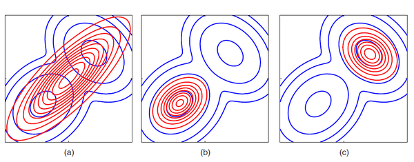
作者:肖天睿鏈接:https://www.zhihu.com/question/29980971/answer/93489660來源:知乎著作權歸作者所有,轉載請聯系作者獲得授權。Interesting question, KL divergence is something I'm working with right now.KL divergence KL(p||q), in the context of information theory, measures the amount of extra bits (nats) that is necessary to describe samples from the distribution p with coding based on q instead of p itself. From the Kraft-Macmillan theorem, we know that the coding scheme for one value out of a set X can be represented q(x) = 2^(-l_i) as over X, where l_i is the length of the code for x_i in bits.We know that KL divergence is also the relative entropy between two distributions, and that gives some intuition as to why in it's used in variational methods. Variational methods use functionals as measures in its objective function (i.e. entropy of a distribution takes in a distribution and return a scalar quantity). It's interpreted as the "loss of information" when using one distribution to approximate another, and is desirable in machine learning due to the fact that in models where dimensionality reduction is used, we would like to preserve as much information of the original input as possible. This is more obvious when looking at VAEs which use the KL divergence between the posterior q and prior p distribution over the latent variable z. Likewise, you can refer to EM, where we decomposeln p(X) = L(q) + KL(q||p)Here we maximize the lower bound on L(q) by minimizing the KL divergence, which becomes 0 when p(Z|X) = q(Z). However, in many cases, we wish to restrict the family of distributions and parameterize q(Z) with a set of parameters w, so we can optimize w.r.t. w.Note that KL(p||q) = - \sum p(Z) ln (q(Z) / p(Z)), and so KL(p||q) is different from KL(q||p). This asymmetry, however, can be exploited in the sense that in cases where we wish to learn the parameters of a distribution q that over-compensates for p, we can minimize KL(p||q). Conversely when we wish to seek just the main components of p with q distribution, we can minimize KL(q||p). This example from the Bishop book illustrates this well.